Given a divergence measure $d(P, Q)$ and two distribution $P$ $Q$, what is the effect to the divergence $d(P^m, Q^m)$ as $m$ increases ? Intuitively, the divergence shall increase since product distribution emphasize the difference of the distribution. In this work by Zinan et.al , the upper and lower bound of $d(P^m, Q^m)$ is given for the divergence measure :
\begin{eqnarray} && d _{p}(P,Q) = \mathop{\sup} _{S} [P(S) - Q(S)] \end{eqnarray}
This measure is closely related to the optimal successful detection probability $P _{\rm opt}$ in the binary hypothesis testing :
\begin{eqnarray}
&& P _{\rm opt} = \mathop{\sup} _{S} [\pi _1 P(S) + \pi _2 (1 - Q(S))] = \pi _2 + d _{p}(\pi _1 P, \pi _2 Q) = \frac{1}{2} + d _{\rm TV}(\pi _1 P, \pi _2 Q)
\end{eqnarray}
where $\pi _1, \pi _2$ are the prior distribution of the hypothesis, and $d _{\rm TV}(P, Q)$ is the total variance distance :
\begin{eqnarray} && d _{TV}(P,Q) = \frac{1}{2} \sum _{\omega \in \Omega} |P(\omega) - Q(\omega)| \end{eqnarray}
What makes the work by Zinan et.al interesting is that if certain local property is satisfied for the distribution pair $(P, Q _1)$ but not for $(P, Q _2)$, and assume $d _p(P, Q _1) = d _p(P, Q _2)$, then the possible value region of $d _p(P^m, Q^m _1)$ splits away from that of $d _p(P^m, Q^m _2)$. This local property is called $(\epsilon, \delta)$ -mode collapse, defined as:
\begin{eqnarray} && P,Q \; {\rm has \; (\epsilon, \delta)- mode \; collapse \; :}\exists S \; {\rm s.t.} \; P(S) \geq \delta \; , Q(S) \leq \epsilon \end{eqnarray}

Interestingly, similar result was given in the quantum literature by Jonas Maziero for trace distance:
\begin{eqnarray} && d _1 (\rho _1, \rho _2) = \frac{1}{2} \Vert \rho _1 - \rho _2 \Vert _1 = {\rm Tr} (\sqrt{(\rho _1 - \rho _2)^{\ast} ( \rho _1 - \rho _2)}) \end{eqnarray}
So, I think it would be fun to dig into the quantum counterpart of Zinan’s work.
A Quantum Counterpart
In the quantum paradigm, the discrete probability distribution is replaced by the density matrix $\rho$, which is a positive semidefinite matrix with trace one. When the matrix is diagonal, it’s reduced back to the classical probability distribution.
For a classical distribution, calculating $P(S)$ for some region $S$ is intuitive and straightforward: It’s the probability of observing events falling within the region $S$. More explicitly, :
\begin{eqnarray} && P(S) = \sum _{\omega \in S} P(\omega) \cdot 1 + \sum _{\omega \notin S} P(\omega) \cdot 0 = \langle P, \mathbb{1} _{S} \rangle \end{eqnarray}
where $\mathbb{1} _S$ is a vector having one on the support $S$ and zero for the other components. This idea is generalized in the quantum domain by quantum measurement. To be more explicit, quantum measurement $\mu$ is a collection of positive semidefinite matrix, such that:
\begin{eqnarray} && \sum _{a \in {\rm some “event” support}} \mu (a) = \mathbb{1} \end{eqnarray}
When measurement is performed on a quantum state $\rho$, event $a$ is selected with probability $\langle \mu (a), \rho \rangle = Tr(\mu (a) ^{\ast} \rho)$. Take the task of binary hypthesis testing as an example, the collection of measurement operator $[\mu (0) , \mu (1)]$ indicates the observation comes from $\rho _{P}$ or $\rho _{Q}$. The successful detection probability is:
\begin{eqnarray} && P _{\rm opt}=\pi _1 \langle \mu (0), \rho _{P}\rangle + \pi _2 \langle \mu (1), \rho _{Q}\rangle \end{eqnarray}
which is further associated with the trace distance (reduce to $d _{TV}$ for classical case), by the well known Holevo-Helstrom theorem:
\begin{eqnarray} && P _{\rm opt}= \pi _1 \langle \mu (0), \rho _{P}\rangle + \pi _2 \langle \mu (1), \rho _{Q}\rangle \leq \frac{1}{2} + \frac{1}{2}\Vert \pi _1 \rho _{P} - \pi _2 \rho _{Q} \Vert _1 \end{eqnarray}
where the equality is established by constructing projective measurement from the Jordan-Hahn decomposition:
\begin{eqnarray} && \pi _1 \rho _{P} - \pi _2 \rho _{Q} = M - N \; , \; \mu^{\ast} (0) = \Pi _{\rm im \; M} \; , \; \mu^{\ast} (1) = \mathbb{1} - \Pi _{\rm im \; M} \end{eqnarray}
where $(M,N)$ are both positive semidefinite, and $\Pi _{\rm im \; M} $ is the projection operator onto the image of $M$. This corresponds to the optimal $S$ given by $d _{p}(\pi _1 P, \pi _2 Q)$ in the case $\rho _{P} \; \rho _{Q}$ are both diagonal.
($\epsilon, \delta$)- mode collapse can be rephrased in a quantum manner. State pair $(\rho _{P}, \rho _{Q})$ has ($\epsilon, \delta$) -mode collapse if there exist a measurement operator $\mathbb{0} \leq \mu(a) \leq \mathbb{1}$ with $a \in \mathcal{A}$ for some collection, such that $\langle \mu (a), \rho _{P}\rangle \geq \delta$ and $\langle \mu (a), \rho _{Q} \rangle \leq \epsilon$.
Theorem statements
Before heading toward some examples in the next section, we first state the theorem by Zinan et.al:
Examples: Binary support
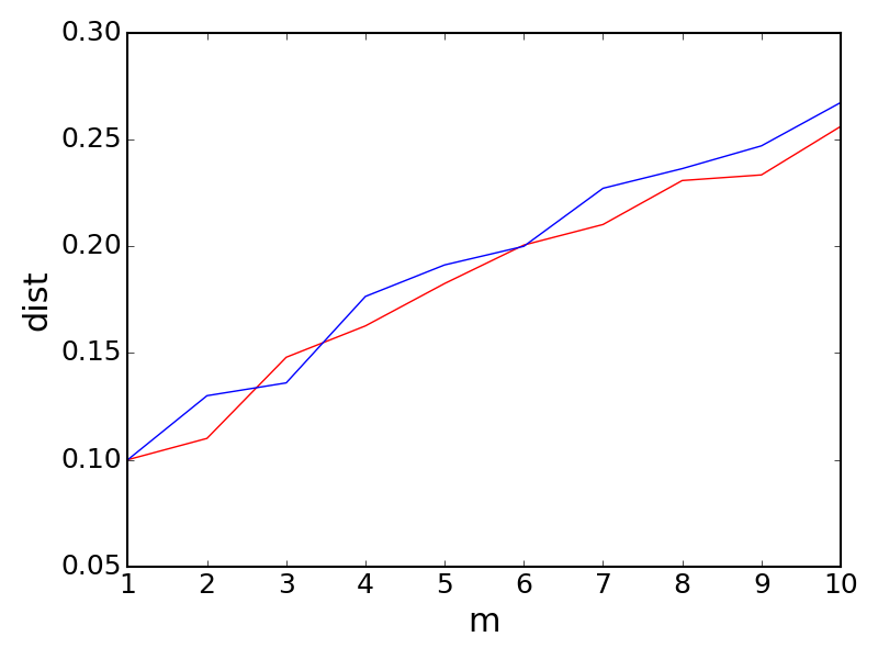
Consider distribution on a binary support. Given total variance, there’re two possible distribution pair. For instance, $P = [0.4, 0.6], Q _1 = [0.3, 0.7], Q _2 = [0.5, 0.5]$, we have that $d _{p} (P,Q _1) = d _p (P, Q _2) = 0.1$, while $(P,Q _1)$ exhibits $(0.3 , 0.4) - $ mode collapse but $(P, Q _2)$ has no such mode collapse. Note that $(P, Q _2)$ has $(0.5, 0.6) - $ mode collapse and $(P, Q _1)$ has no such mode collapse. The simulation result is given below :
As for the quantum case, things start to become more ineteresting. First, a two dimensional quantum state has three degree of freedom, which makes all the $\rho _x$ with the same $d _1(\rho, \rho _x)$ to be more than that of the classical case. Second, there are more possibilities (e.g. all the density matrices) for the mode collapse ‘region’ than the classical case ($\mu _0 = \vert 0 \rangle \langle 0 \vert \; , \; \mu _1 = \vert 1 \rangle \langle 1 \vert$).
For example, \begin{eqnarray} && \rho _{P} = \begin{pmatrix} \frac{1}{2} & 0 \newline 0 & \frac{1}{2} \end{pmatrix} \newline && \rho _{Q _1} = \begin{pmatrix} \frac{1}{2} & \frac{1}{2} \newline \frac{1}{2} & \frac{1}{2} \end{pmatrix} \newline && \rho _{Q _2} = \begin{pmatrix} 1 & 0 \newline 0 & 0 \end{pmatrix} \end{eqnarray}
The trace distance $0.5 \cdot \Vert \rho _{P} - \rho _{Q _1} \Vert _1 = 0.5 \cdot \Vert \rho _{P} - \rho _{Q _2} \Vert _1 = 0.5 $. Now classically, given $\mu (0) = \vert 0 \rangle \langle 0 \vert \; , \; \mu (1) = \vert 1 \rangle \langle 1 \vert$ , $(\rho _{P}, \rho _{Q _2})$ exhibits $(0, 1/2)$-mode collapse while $(\rho _{P}, \rho _{Q _1})$ doesn’t. However, trace distance $d _1 ( \rho _{P}^m, \rho _{Q _1} ^m )$ and $d _1( \rho _{P}^m, \rho _{Q _2} ^m )$does not split as $m$ increases. In fact, careful calculation leads to : \begin{eqnarray} && d _1(\rho _P ^m, \rho _{Q _1} ^m) = d _2(\rho _P ^m, \rho _{Q _2} ^m ) = (1 - \frac{1}{2 ^m}) \end{eqnarray}
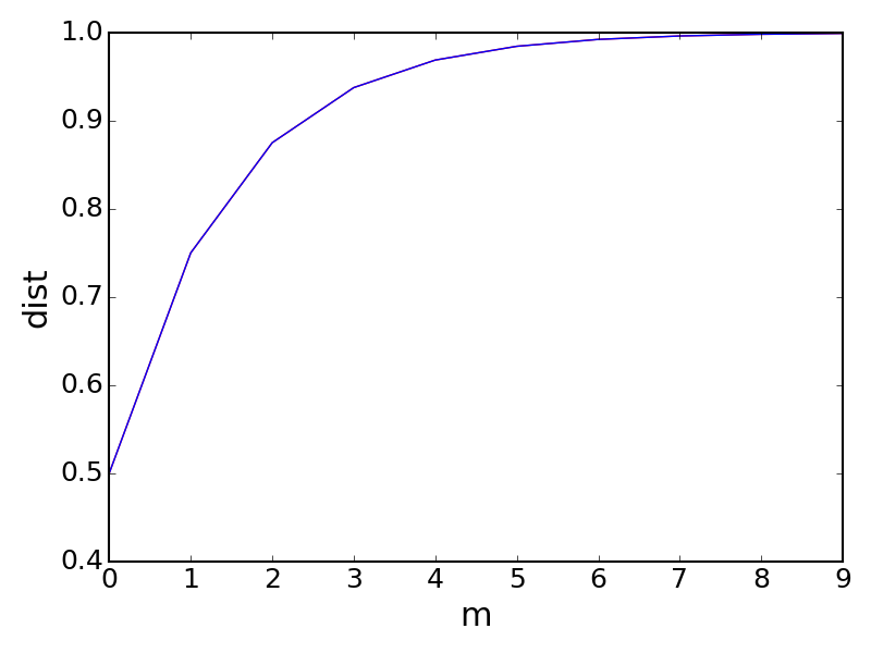
But if we consider the quantum definition for mode collapse, we can see that both $(\rho _P, \rho _{Q _1})$ and $(\rho _P, \rho _{Q _2})$ exhibits $(0 , 1/2)$ mode collapse, and the latter mode collapse is achieved when $\mu = \begin{pmatrix} \frac{1}{2} & \frac{-1}{2} \newline \frac{-1}{2} & \frac{1}{2}\end{pmatrix}$. In fact, under the Bloch sphere representation, $(\rho _P, \rho _{Q _1})$ and $(\rho _P, \rho _{Q _2})$ are identical up to a unitary transform. To be more explicit, any two-dimensional quantum state $\rho$ (pure or mixed) can be represented in the Bloch representation:
\begin{eqnarray} && \rho = \frac{\mathbb{1} + \vec{r} \cdot \vec{\sigma}}{2} \newline && \vec{r} \in \mathbb{R}^3 \; , \; \Vert \vec{r} \Vert _2 \leq 1 \newline && \vec{\sigma} = (\sigma _x, \sigma _y, \sigma _z) \end{eqnarray}
where $(\sigma _x, \sigma _y, \sigma _z)$ are the Pauli matrices. When $\vec{r} = \vec{0}$, it’s called a completely mixed state; when $\Vert \vec{r} \Vert _2 = 1$, it’s pure state. Notably, the trace distance between two arbitrary two-dimensional quantum state is:
\begin{eqnarray} && d _1(\rho _1, \rho _2) = \frac{\Vert \vec{r} _1 - \vec{r} _2\Vert _2}{2} \end{eqnarray}
Also, trace distance is unitarily invariant : $d _1(\rho _1, \rho _2) = d _1(U \rho _1 U ^{\ast}, U \rho _2 U ^{\ast})$. So the above example is a special case for the following theorem:
One can check that when $\Vert \vec{r} \Vert _2 = 1$, $d _1(\rho _0 ^m , \rho _r ^m) = 1 - \frac{1}{2 ^m}$, which coincides with the result.
To show a signficant distance split in 2 dimensional cases, we consider the example in the following figure. It shows the possible region of $d _1(\rho ^m, \rho _x ^m)$ among all possible $\rho _x$ such that $d _1(\rho, \rho _x ) = 0.25$, and $\rho$ is randomly selected on a $0.5-$ radius Bloch sphere.
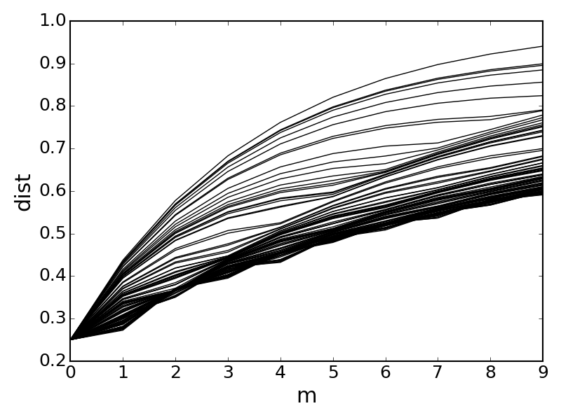
To coincide the split with Zinan’s work, we adopts the geometric approach as in Zinan’s original paper. We’d like to see what is the quantum counterpart and characterisitc of the so called mode collapse region.
Mode collapse region
Mode collapse region is defined as :
Likewise, a quantum counterpart for mode collapse region can be defined as:
Let’s investigate both the classical and quantum mode collaspe region for binary support distribution. Consider the example $(P,Q_1)$ in the previous section, the classical mode collapse region is plotted as below:
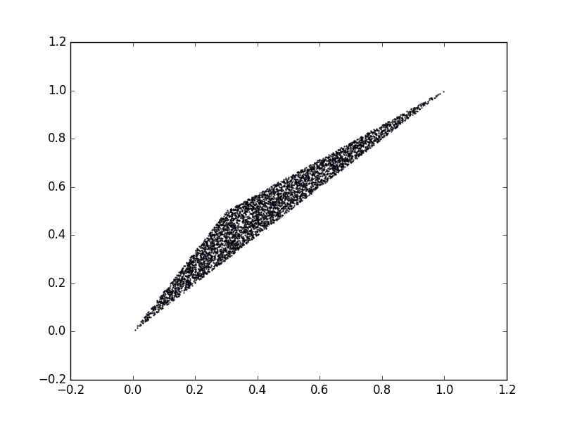
And the quantum mode collapse region is plotted as below:

As from the experiment result, both the classical and quantum mode collapse region are the same. In fact, we can prove the following theorem:
How do we associate the mode collapse region with the divergence bound ? In Zinan’s work, he first observe that if $\mathcal{R} (P _1,Q _1) \subset \mathcal{R} (P _2, Q _2) $, then $d _p(P _1,Q _1) \leq d _p(P _2, Q _2)$. Thus, the problem of bounding divergence is associated with bounding the mode collpase region.
Furthermore, a key lemma for bounding the mode collapse region is resulted from an implication of the Blackwell’s theorem :
\begin{eqnarray} && \mathcal{R} (P _1, Q _1) \subset \mathcal{R} (P _2, Q _2) \rightarrow \mathcal{R} (P _1 ^m, Q _1 ^m) \subset \mathcal{R} (P _2 ^m, Q _2 ^m) \; \forall \; m \end{eqnarray}
Interestingly, a quantum counterpart of the Blackwell’s theorem: _ the Shmaya’s theorem leads to a same implication for quantum mode collapse region. We can prove that:
Combining the above two theorem, the bound obtained by Zinan in the classical literature is actually applicable for the quantum case. For instance, consider the last experiment in the previous section, we can almost tightly bound all the possible value region for $d _1 (\rho ^m, \rho _x ^m )$ with $\rho _x$ satisfying $d _1(\rho, \rho _x) = 0.25$:
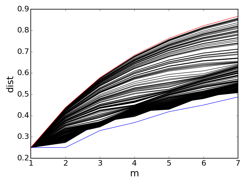
As the result, all the split phenomenon caused by mode collapse in the classical setting can be adopted in the quantum counterpart.