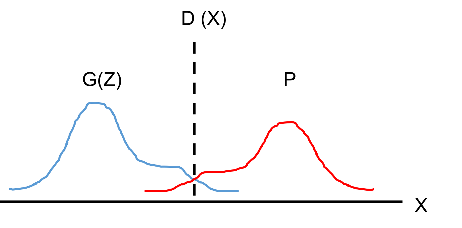
Recently a bunch of Generative Adversarial Net (GAN) related research has boomed in the unsupervised learning community, and it seems interesting to fully understand the mechanism of this novel learning framework. Just a few days ago (July 5th, 2018), Alexia Jolicoeur-Martineau et al proposed a Relativistic GAN that aimed to provide improvement via changes of the discriminator term in the original GAN objective function. It pointed out that the real data are usually ignored during the learning process in most GAN paradigm, and thus it proposed a relativistic quantity to measure how ‘real’ the real samples are compared to the fake sample.

It seems to to me that the original goal of GAN is to train the followings given the sampled real data sets $x_i \mathop{\sim}^{i.i.d} P$:

• A generator $G_{\theta}(z)$ that has small distributional divergence with respect to the true distribution. This is the main goal of the generative learning paradigm.

• A discriminator $D_{\omega}$ equipped with strong detection ability. This is rather a side product for GAN, but the training procedure relies on the detection result (e.g. the backpropagation for weight update.)

Generator perspective: minimization of the divergence

For the first part, most GAN objective functions are some $f$ divergence with the following forms:

\begin{eqnarray} && D_f(P||Q) = \int_{\chi} q(x)f \Big( \frac{p(x)}{q(x)}\Big) dx \end{eqnarray}

As pointed out in the $f$ GAN literature, the $f$ divergence is approximated via a variational lower bound known as Frenchel conjugate $f^\ast$ (for all lower-semicontious function $f$). This conjugate is convex with the defintion:

\begin{eqnarray} && f^\ast (t) = \mathop{\sup}_{u \in {\rm dom}_f} [ut - f(u)] \end{eqnarray}

Likewise, $f$ can be expressed in terms of $f^\ast$ since the pair $(f, f^\ast)$ are dual to each other. Plugging into the expression of the $f$ divergence, we have:

\begin{eqnarray} && D_f(P||Q) = \int_{\chi} q(x) \mathop{\sup}_{t \in {\rm dom} _{f^\ast}} \Big( t\frac{p(x)}{q(x)} - f^\ast(t) \Big) dx \newline && \geq \sup _{T(x) \in \mathcal{T}} \Big( \int _{\chi} p(x) T(x) dx - \int _{\chi} q(x) f^\ast (T(x)) \Big) \newline && = \sup _{T(x) \in \mathcal{T}} (E _{x \sim P}[T(x)] - E _{x \sim Q}[f^ \ast (T(x))]) \end{eqnarray}

To achieve the tightest lower bound, $T(x) = \frac{df}{dx} \big(\frac{p(x)}{q(x)}\big)$. For instance, consider a $f$ divergence with $f(u) = u \log u - (u+1) \log (u+1)$, first compute the Frenchel dual as :

\begin{eqnarray} && f^\ast (t) = \mathop{\sup} _{u > 0} [ut - u \log u + (u+1) \log(u+1)] \newline && = - (t + \log (10^{-t} - 1)) \; , \; t < 0 \end{eqnarray}

So the variational lower bound for the $f$ divergence becomes :

\begin{eqnarray} && \sup _{T(x) \in \mathcal{T}} (E _{x \sim P}[T(x)] + E _{x \sim Q}[\log (1 - exp(T(x)))]) \end{eqnarray}

Standard GAN adopts $T(x)$ with the form :

\begin{eqnarray} && T(x) = \log D_\omega(x) = 1/(1 + e^{-V_{\omega}(x)}) \end{eqnarray}

So the loss is the familiar form :

\begin{eqnarray} && L(\theta, \omega) = \mathop{\sup} _{D} [E _{x \sim P}[\log D _{\omega}(x)] + E _{x \sim G _{\theta}(P_z)}[\log (1 - D _{\omega}(x))]] \end{eqnarray}

When $D(x)$ is optimal, it has $D(x) = \frac{p(x)}{p(x) + G_{\theta} (P_z)(x)}$, or with $Q_{\theta} = G_{\theta}(P_z)$ as a shorthand, $D(x) = \frac{p(x)}{p(x) + q_{\theta}(x)}$. Plugging it back to the variational bound, one can recover the J-S divergence in the literature. Thus with a perfect discriminator, the generator can be trained to minimize the divergence loss between generated distribution and the target distribution.

Discriminator perspective: Optimal Detector

The above arguments stand on a generator perspective, where the goal is to minmize a divergence measure (with high fidelity). On the other hand, we’ve seen that the optimal discriminator to construct JS divergence is actually a maximum likelihood detector. ML is also an optimal detector for hypthothesis testing with uniform prior, where the performance metric is the Bayesian risk. Such a correspondence between divergence measure and the optimal Bayesian detector is not a coincidence: The form of the standard GAN variational lower bound takes a log-likelihood expression. i.e, when jointly maximize the log of true alarm and negative probability, one get a J-S divergence measure with a Bayesian optimal detector.

For more example, consider a variational objective with $0-1$ loss, i.e.,

\begin{eqnarray} && L(\theta, \omega) = \mathop{\sup} _{D : \chi \to 0, 1} [ E _{x \sim P}[\mathbb{1}[D _{\omega}(x)]] + E _{G _{\theta}(z) \sim Q}[1 - \mathbb{1}[D _{\omega}(G _{\theta}(x))]]] \end{eqnarray}

This loss is exactly (up to a 1/2 prior probability) related to the Bayesian risk, and the maximization of it leads to a divergence measure called total variance $d_{\rm TV}(P,Q)$, defined as:

\begin{eqnarray} && d_{\rm TV}(P,Q) = \mathop{\sup}_{S \subset \chi} [P(S) - Q(S)] = L(\theta, \omega^\ast) - 1 \end{eqnarray}

So to construct an optimal detector in a sense of the Baysian risk, the discriminator should jointly maximize the true positive and negative probability. And its maximum is $1 + d _{\rm TV}(P,Q)$. Likewise, standard GAN jointly maximize the log likelihood of true positive and negative probabilty, which yields an optimal value expressed by the J-S divergence. For other GAN, one can also trace the decision region of the optimal discriminator, and may understand if such a GAN bias toward true positive or true negative probability.

Dose GAN bias toward true positive or true negative during the training process ?